Introduction
During Breakthrough Listen observations we record coarsely-channelized complex voltage data to GUPPI raw files. We do this because we further channelize the data into a number of different data products: a high-frequency resolution, low-time resolution narrow-band search product, a high-time resolution, low-frequency resolution transient pulse product, and a integrated spectrum for traditional radio observations. The complex voltage data represents the rawest form of the data. When our processing pipelines report an interesting detection we can go back to the original data as it provides the most information available. This is the case for FRB 180301 which was detected in a incoherent search survey with the Parkes Telescope. We can coherently dedisprse the complex voltages to improve the time and frequency resolution, and reduce the effects of smearing to increase the Signal-to-Noise (S/N). This is a short tutorial on going through this process.
Pre-requisites
We will need a few bits of software and the original data to get going:
We will use dspsr to perform the coherent dedispersion and we will use the digihdr utility to print the GUPPI raw header.
git clone https://github.com/UCBerkeleySETI/dspsr
cd dspsr
vim backends.list
Add the following backends: fits guppi sigproc
./bootstrap
./configure
make -j
make install
We will use psrchive with the archive files output by dspsr to apply calibration, zap RFI, and fit a rotation measure.
git clone git://git.code.sf.net/p/psrchive/code psrchive
cd psrchive
./bootstrap
./configure --enable-shared F77=gfortran FFLAGS=-fPIC CFLAGS=-fPIC
make -j
make install
We will use the Breakthrough Listen python file interface module (blimpy) to get some additional information from the file headers.
pip install blimpy
Or, for the latest development version:
pip install https://github.com/UCBerkeleySETI/blimpy/tarball/master
Last, we need the data:
- Upper-band GUPPI raw: extracted_58178_27040_085674_FRB180301_0001.raw
- Lower-band GUPPI raw: extracted_58178_27040_085674_FRB180301_0001.raw
- Calibration observation: CAL.ar
TODO: data links
Determining the Observation Meta-data
We need to determine a few parameters of the raw data so that we can generate a reasonable dynamic spectrum. Using blimpy we find the time resolution of the sampled complex voltages to be ~285 ns (this is because the coarse channelization in the BL front-end produces approximately 3.5 MHz wide channels), there are 44 of these channels per raw file:
> ipython
> import blimpy
> r = blimpy.GuppiRaw('upper_halfband/extracted_58178_27040_085674_FRB180301_0001.raw')
> r.read_header()

...
'OBSNCHAN': 44,
...
'TBIN': 2.8571428571429e-07,
...
We need the number of time samples (2621440) to determine the total time of the file and number of ‘phase bins’ to channelize the data to. We will set the total time length to be a single ‘period’ of the pulse, so the phase will go from 0 to 1 across the file.
> digihdr extracted_58178_27040_085674_FRB180301_0001.raw

ndat             Number of time samples         2621440
nchan            Number of frequency channels   44
npol             Number of polarizations        2
ndim             Number of data dimensions      2
nbit             Number of bits per datum       8
type             Observation type               Pulsar
site             Telescope name                 PARKES
name             Source name                    G204.17-6.06
coord            Source coordinates             06:12:43.464+04:33:44.28
freq             Centre frequency (MHz)         1436.75
bw               Bandwidth (MHz)                -154
dm               Dispersion measure (pc/cm^3)   0
rm               Rotation measure (rad/m^2)     0
scale            Data units                     1
state            Data state                     Analytic
The total time length of the file is 0.7489828571428683 seconds.
Coherently Dedispersion
Now we are ready to coherently dedisperse the data. The dispersion measure which optimizes the S/N of the pulse has been found to be 522.0 pc cm^-3. The default file format output of dspsr is a psrchive file.
dspsr -T 0.7489828571428683 -c 0.7489828571428683 -cepoch 58178 -O FRB180301_upper -D 522.0 -d 4 -b 32768 -K -F 1408:D -p 0 upper_halfband/extracted_58178_27040_085674_FRB180301_0001.raw
dspsr -T 0.7489828571428683 -c 0.7489828571428683 -cepoch 58178 -O FRB180301_lower -D 522.0 -d 4 -b 32768 -K -F 1408:D -p 0 lower_halfband/extracted_58178_27040_085674_FRB180301_0001.raw
- -T
-c : set the total processed time and period to be the length of the file. - -cepoch
: reference MJD to set phase=0 - -O
: output filename without the filetype extension - -D
: dispersion measure - -d
: number of polarizations, 4 to produce complete coherency products - -b
: number of phase bins, should be a multiple of the number of time samples, e.g. 2621440/80 = 32768, ~22 microsecond resolution per spectra - -F
:D : number of channels per spectrum, should be a multiple of the number of coarse channels, e.g. 44*32 = 1408, ~109.375 kHz resolution
Plot the Dynamic Spectrum
We can plot the dynamic spectrum of these archive files with psrplot
psrplot -p freq+ -D /xs -c 'x:unit=ms,x:range=(0.575,0.6)' FRB180301_upper.ar
- -p freq+: plot the dynamic spectrum, the frequency-integrated profile, and the time-integrated spectrum
- -D /xs: plot figure to screen
- -c ‘x:unit=ms,x:range=(0.575,0.6)’: show the x-axis as a time in milliseconds over a phase range (0.575,0.6)
Instead of plotting the figure to screen, the figure can be written to file by changing the device:
psrplot -p freq+ -D FRB180301_upper_0.png/png -c 'x:unit=ms,x:range=(0.575,0.6)' FRB180301_upper.ar
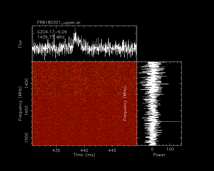
The pulse isn’t clear in the dynamic spectrum, but can be seen in the frequency-integrated profile. There is no apparent flux in the lower band.
Polarization Calibration
The archive file we generated is uncalibrated, the amplitudes are just related to the digital gain of the front-end. We need to apply some calibration, particularly polarization calibration so that we can generate correct Stokes parameters. To do this a calibration observation needs to be performed, luck for us, that has all ready happened. We will use the CAL.ar file. From psrsh we will generate a calibration file for each band.
psrsh
> load CAL.ar
> delete freq <1359.75
> delete freq >1513.75
> scale -1 pol[3]
> edit bw=-154
> edit freq=1436.75
> edit be:name=GUPPI
> edit rcvr:name=BL
> unload CAL.blh
Or, the commands can be written in a script and executed by command line (exclude the load line),
./prepCalUpper.sh CAL.ar
For the upper band we select the frequency band, and set the bandwidth and centre frequency. There is a phase convention correction that needs to be set by flipping the Stokes V phase. Then the calibration file will be written to CAL.blh. We use pac to apply the calibration:
pac -w -u blh
pac -T -d database.txt FRB180301_upper.ar
The first line generates a new database file based on the blh file extension. The second line applies that database file to the archive and writes out a new file with the calibP extension. Then, we do the same for the lower band,
psrsh
> load CAL.ar
> delete freq >1359.75
> delete freq <1205.75
> scale -1 pol[3]
> edit bw=-154
> edit freq=1282.75
> edit be:name=GUPPI
> edit rcvr:name=BL
> unload CAL.bll
./prepCalLower.sh CAL.ar
pac -w -u bll
pac -T -d database.txt FRB180301_lower.ar
Zap RFI Channels
There are few channels in the lower band with consistent, known RFI, so we mask (zap) them out:
psrsh
> load FRB180301_lower.calibP
> zap freq 1206:1208
> zap freq 1245.5:1246.5
> zap freq 1265:1273
> unload ext=rfi
Or, write the commands as a script,
./zapRFI.sh FRB180301_lower.calibP
This outputs a new lower band archive file with a .rfi extension.
Rotation Measure Fitting
Since the data contains full Stokes information, we can do a rotation measure fit to the pulse. Only the upper band contains significant flux, so we will only perform the fit on that portion of the band.
rmfit -t -a 1 -A 1 -B 32 -F 2 -D -K rmfit.png/png FRB180301_upper.calibP >& rmfit.log &
- -t: use the default RM range and step size
- -a
: step size based on delta-Psi in radians - -A
: set the maximum RM base on a similar criteria to -a option - -B
: scrunch the number of phase bins by this factor - -F
: scrunch the number of frequency channels by this factor - -D : display results
- -K : device to write figure to
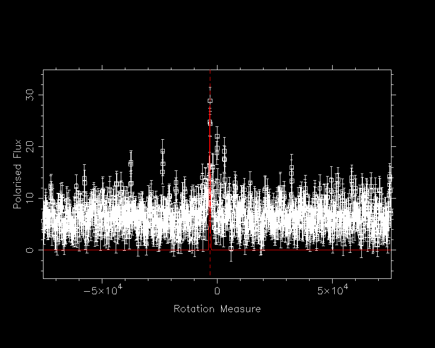
Based on the RM fit there is a peak at -3163.21, this can be found in the rmfit.log file. The pam program can be used to apply this rotation measure and output rotation measure corrected archives with a .RM extension.
pam -R -3163.21 -e RM FRB180301_upper.calibP
pam -R -3163.21 -e RM FRB180301_lower.rfi
Where to go next
Now we have coherently dedispersed, polarization calibrated, RFI zapped, rotation measure corrected dynamic spectra. From here there are a umber of pths to go down. One of the most convenient is to use the psrchive python interface to load the files into numpy arrays.